(Solved): For a function f:R^(d)->R, a point x_(0) is a locel minimum if there exists \delta >0 such tha ...
For a function
f:R^(d)->R, a point
x_(0)is a locel minimum if there exists
\delta >0such that for all
xwith
||x-x_(0)||<\delta ,f(x_(0))<=f(x). Similarly, a point
x_(0)is a local maximum if the opposite holds: if there exists
\delta >0such that for all
xwith
||x-x_(0)||<\delta ,f(x_(0))>=f(x). There exist smooth functions for which finding a local minimum is NP-hard. However, if
fis differentiable, then one necessary condition for
x_(0)to be a local minimum is that
gradf(x_(0))=0. (a) This is necessary but not sufficient! Give an example of a function in two dimensions and a point
x_(0)such that
gradf(x_(0))=0but
x_(0)is neither a local minimum nor a local maximum of
f. [1 points] (b) Inspite of the above, vanishing gradients is often desired. Suppose we have a
\beta -smooth function
f:R^(d)->R. Show that gradient descent can be used to find a point
wsuch that
||gradf(w)||<=\epsi . How many iterations of GD do you need for finding such a point? Your bound can depend on the starting point,
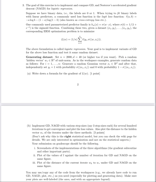
f(w_(0)),\beta ,\epsi , and the value of the glolbal optimum (which you can assume is bounded). [2 points] 1 [Hint: Try to use the monotonicity property of GD and combine all the equations over the iterates.] The goal of this exercise is to implement and compare GD, and Nesterov's accelerated gradient descent (NAGD) for logistic regression. Suppose we have binary data, i.e., the labels are 0 or 1 . When trying to fit binary labels with linear predictors, a commonly used loss function is the logit loss function:
l(a,b)=
-alogb-(1-a)log(1-b)(also known as cross-entropy loss etc.). One commonly used parameterized predictor family is
h_(w)(x)=\sigma (w*x), where (
:e^(-t)