Home /
Expert Answers /
Mechanical Engineering /
table-2-problem-specific-parameters-in-the-end-you-have-4-states-x-x-x-theta-theta-pa478
(Solved): Table 2: Problem specific parameters. In the end, you have 4 states x=(x,x^(),\theta ,\theta ^() ...
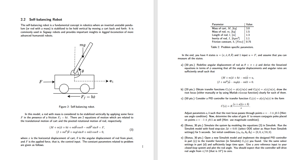
Table 2: Problem specific parameters.
In the end, you have 4 states x=(x,x^(?),\theta ,\theta ^(?)) and 1 input u=F. and assume that you can
measure all the states.
a\theta =\pi +\phi and derive the linearized
equations in terms of \phi assuming that all the angular displacements and angular rates are
sufficiently small such that
(M+m)tilde(x)+bx^(?)-ml\phi ^(¨)=u,
(I+ml^(2))\phi ^(¨)-mgl\phi
(t)ml=0.
bG_(1)(s)=\phi (s)/(u)(s) and G_(2)(s)=x(s)/(u)(s), draw the
root locus (either manually or by using Matlab rlocus function) clearly for each of them.
cG_(1)(s)=\phi (s)/(u)(s) in the form
C(s)=K((s+a)(s+b))/(s)
Adjust parameters a,b such that the root locus passes through points s=-1+-j0.5 (Hint:
use angle condition). Now, determine the value of gain K to ensure conjugate poles placed
on points s=-1+-j0.5 as well (Hint: use magnitude condition).
d\Delta t=0.01{:x_(0),x_(0)^(?),\theta _(0),\theta _(0)^(?))=(0,0,(\pi )/(18),0).
eG_(1)(s) you found. Use the same solver
settings in part (d) and sufficiently large time span. Give a zero reference input to your
closed-loop system and plot the rod angle. You should expect that the controller will drive
rod angle from (\pi )/(18)10\deg