(Solved): Use improved Euler's method to obtain a four-decimal approximation of the indicated value. First, us ...

Use improved Euler's method to obtain a four-decimal approximation of the indicated value. First, use h=0.1, and then use h=0.05.

Improved Euler's Method (from textbook):

 

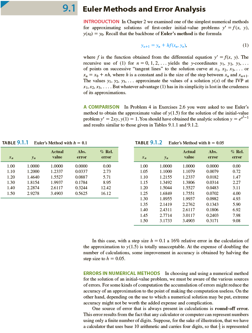
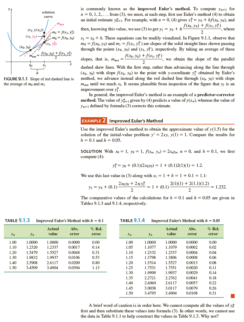
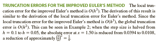
\( y^{\prime}=x^{2}+y^{2}, \quad y(0)=1 \) 9. I Euler Methods and Error Analysis INTRODUCTION In Chapter 2 we examined one of the simplest numerical methods for approximating solutions of first-order initial-value problems \( y^{\prime}=f(x, y) \), \( y\left(x_{0}\right)=y_{0} \). Recall that the backbone of Euler's method is the formula \[ y_{n+1}=y_{n}+h f\left(x_{n}, y_{n}\right) \] where \( f \) is the function obtained from the differential equation \( y^{\prime}=f(x, y) \). The recursive use of (1) for \( n=0,1,2, \ldots \) yields the \( y \)-coordinates \( y_{1}, y_{2}, y_{3}, \ldots \) of points on successive "tangent lines" to the solution curve at \( x_{1}, x_{2}, x_{3}, \ldots \) or \( x_{n}=x_{0}+n h \), where \( h \) is a constant and is the size of the step between \( x_{n} \) and \( x_{n+1} \). The values \( y_{1}, y_{2}, y_{3}, \ldots \) approximate the values of a solution \( y(x) \) of the IVP at \( x_{1}, x_{2}, x_{3}, \ldots \). But whatever advantage (1) has in its simplicity is lost in the crudeness of its approximations. A COMPARISON In Problem 4 in Exercises \( 2.6 \) you were asked to use Euler's method to obtain the approximate value of \( y(1.5) \) for the solution of the initial-value problem \( y^{\prime}=2 x y, y(1)=1 \). You should have obtained the analytic solution \( y=e^{x^{2}-1} \) and results similar to those given in Tables 9.1.1 and 9.1.2. TABLE 9.1.1 Euler's Method with \( h=0.1 \) TABLE 9.1.2 Euler's Method with \( h=0.05 \) In this case, with a step size \( h=0.1 \) a \( 16 \% \) relative error in the calculation of the approximation to \( y(1.5) \) is totally unacceptable. At the expense of doubling the number of calculations, some improvement in accuracy is obtained by halving the step size to \( h=0.05 \). ERRORS IN NUMERICAL METHODS In choosing and using a numerical method for the solution of an initial-value problem, we must be aware of the various sources of errors. For some kinds of computation the accumulation of errors might reduce the accuracy of an approximation to the point of making the computation useless. On the other hand, depending on the use to which a numerical solution may be put, extreme accuracy might not be worth the added expense and complication. One source of error that is always present in calculations is round-off error. This error results from the fact that any calculator or computer can represent numbers using only a finite number of digits. 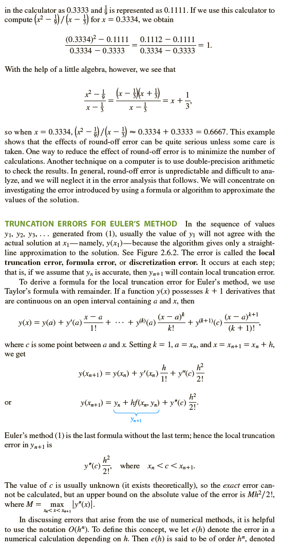Suppose, for the sake of illustration, that we have a calculator that uses base 10 arithmetic and carries four digits, so that \( \frac{1}{3} \) is represented in the calculator as \( 0.3333 \) and \( \frac{1}{9} \) is represented as \( 0.1111 \). If we use this calculator to compute \( \left(x^{2}-\frac{1}{9}\right) /\left(x-\frac{1}{3}\right) \) for \( x=0.3334 \), we obtain \[ \frac{(0.3334)^{2}-0.1111}{0.3334-0.3333}=\frac{0.1112-0.1111}{0.3334-0.3333}=1 . \] With the help of a little algebra, however, we see that \[ \frac{x^{2}-\frac{1}{9}}{x-\frac{1}{3}}=\frac{\left(x-\frac{1}{3}\right)\left(x+\frac{1}{3}\right)}{x-\frac{1}{3}}=x+\frac{1}{3} \] so when \( x=0.3334,\left(x^{2}-\frac{1}{9}\right) /\left(x-\frac{1}{3}\right) \approx 0.3334+0.3333=0.6667 \). This example shows that the effects of round-off error can be quite serious unless some care is taken. One way to reduce the effect of round-off error is to minimize the number of calculations. Another technique on a computer is to use double-precision arithmetic to check the results. In general, round-off error is unpredictable and difficult to analyze, and we will neglect it in the error analysis that follows. We will concentrate on investigating the error introduced by using a formula or algorithm to approximate the values of the solution. TRUNCATION ERRORS FOR EULER'S METHOD In the sequence of values \( y_{1}, y_{2}, y_{3}, \ldots \) generated from (1), usually the value of \( y_{1} \) will not agree with the actual solution at \( x_{1} \)-namely, \( y\left(x_{1}\right) \)-because the algorithm gives only a straightline approximation to the solution. See Figure 2.6.2. The error is called the local truncation error, formula error, or discretization error. It occurs at each step; that is, if we assume that \( y_{n} \) is accurate, then \( y_{n+1} \) will contain local truncation error. To derive a formula for the local truncation error for Euler's method, we use Taylor's formula with remainder. If a function \( y(x) \) possesses \( k+1 \) derivatives that are continuous on an open interval containing \( a \) and \( x \), then \[ y(x)=y(a)+y^{\prime}(a) \frac{x-a}{1 !}+\cdots+y^{(k)}(a) \frac{(x-a)^{k}}{k !}+y^{(k+1)}(c) \frac{(x-a)^{k+1}}{(k+1) !} \] where \( c \) is some point between \( a \) and \( x \). Setting \( k=1, a=x_{n} \), and \( x=x_{n+1}=x_{n}+h \), we get \[ \begin{array}{l} y\left(x_{n+1}\right)=y^{y\left(x_{n}\right)+y^{\prime}\left(x_{n}\right)} \frac{h}{1 !}+y^{\prime \prime}(c) \frac{h^{2}}{2 !} \\ y\left(x_{n+1}\right)=\underbrace{y_{n}+h f\left(x_{n}, y_{n}\right)}_{y_{n+1}}+y^{\prime \prime}(c) \frac{h^{2}}{2 !} . \end{array} \] or Euler's method (1) is the last formula without the last term; hence the local truncation error in \( y_{n+1} \) is \[ y^{\prime \prime}(c) \frac{h^{2}}{2 !} \text { ! where } \quad x_{n}