(Solved): USE MATLAB, USE MATLAB, USE MATLAB, USE MATLAB, USE MATLAB!!!!!!!!!!!!!!!!!!!!!!!!!!!!!!!!!!!!!!!!!! ...

USE MATLAB, USE MATLAB, USE MATLAB, USE MATLAB, USE MATLAB!!!!!!!!!!!!!!!!!!!!!!!!!!!!!!!!!!!!!!!!!!!!!!!!!!!!!!!

DO NOT ANSWER THIS QUESTION WITHOUT MATLAB

USE MATLAB TO PLOT THE WAVEFORMS SHOWN IN FIGURE 2.3. I WILL GIVE A DISLIKE IF NO MATLAB CODE IS PROVIDED AND NO WAVEFORM GENERATED BY MATLAB

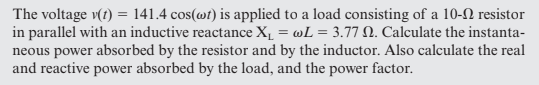
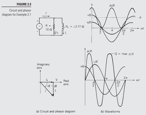
The voltage \( v(t)=141.4 \cos (\omega t) \) is applied to a load consisting of a \( 10-\Omega \) resistor in parallel with an inductive reactance \( \mathrm{X}_{\mathrm{L}}=\omega L=3.77 \Omega \). Calculate the instantaneous power absorbed by the resistor and by the inductor. Also calculate the real and reactive power absorbed by the load, and the power factor. 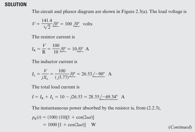FIGURE \( 2.3 \) Circuit and phasor diagram for Example \( 2.1 \) (a) Circuit and phasor diagram (b) Waveforms The circuit and phasor diagram are shown in Figure 2.3(a). The load voltage is \( V=\frac{141.4}{\sqrt{2}} \angle 0^{\circ}=100 \angle 0^{\circ} \) volts The resistor current is \[ I_{\mathrm{R}}=\frac{V}{\mathrm{R}}=\frac{100}{10} \angle 0^{\circ}=10 \angle 0^{\circ} \mathrm{A} \] The inductor current is \[ I_{\mathrm{L}}=\frac{V}{j X_{\mathrm{L}}}=\frac{100}{(j 3.77)} \angle 0^{\circ}=26.53 \angle-90^{\circ} \quad \mathrm{A} \] The total load current is \[ I=I_{\mathrm{R}}+I_{\mathrm{L}}=10-j 26.53=28.35 L-69.34^{\circ} \quad \mathrm{A} \] The instantaneous power absorbed by the resistor is, from (2.2.3), \[ \begin{aligned} p_{\mathrm{R}}(t) &=(100)(10)[1+\cos (2 \omega t)] \\ &=1000[1+\cos (2 \omega t)] \quad W \end{aligned} \] (Continued) 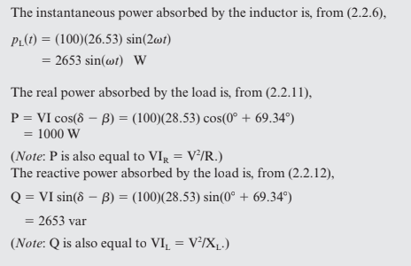The instantaneous power absorbed by the inductor is, from \( (2.2 .6) \), \[ \begin{aligned} p_{\mathrm{L}}(t) &=(100)(26.53) \sin (2 \omega t) \\ &=2653 \sin (\omega t) \quad \mathrm{W} \end{aligned} \] The real power absorbed by the load is, from (2.2.11), \[ \begin{aligned} \mathrm{P} &=\mathrm{VI} \cos (\delta-\beta)=(100)(28.53) \cos \left(0^{\circ}+69.34^{\circ}\right) \\ &=1000 \mathrm{~W} \end{aligned} \] (Note: \( \mathrm{P} \) is also equal to \( \mathrm{VI}_{\mathrm{R}}=\mathrm{V}^{2} / \mathrm{R} \).) The reactive power absorbed by the load is, from (2.2.12), \[ \begin{aligned} Q &=V I \sin (\delta-\beta)=(100)(28.53) \sin \left(0^{\circ}+69.34^{\circ}\right) \\ &=2653 \text { var } \end{aligned} \] (Note: \( \mathrm{Q} \) is also equal to \( \mathrm{VI}_{\mathrm{L}}=\mathrm{V}^{2} / \mathrm{X}_{\mathrm{L}} \).) 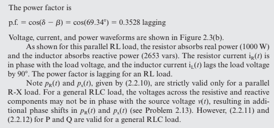The power factor is p.f. \( =\cos (\delta-\beta)=\cos \left(69.34^{\circ}\right)=0.3528 \) lagging Voltage, current, and power waveforms are shown in Figure 2.3(b). As shown for this parallel RL load, the resistor absorbs real power (1000 W) and the inductor absorbs reactive power (2653 vars). The resistor current \( \mathrm{i}_{\mathrm{R}}(t) \) is in phase with the load voltage, and the inductor current \( \mathrm{i}_{\mathrm{L}}(t) \) lags the load voltage by \( 90^{\circ} \). The power factor is lagging for an RL load. Note \( p_{\mathrm{R}}(t) \) and \( p_{\mathrm{x}}(t) \), given by (2.2.10), are strictly valid only for a parallel \( \mathrm{R}-\mathrm{X} \) load. For a general RLC load, the voltages across the resistive and reactive components may not be in phase with the source voltage \( v(t) \), resulting in additional phase shifts in \( p_{\mathrm{R}}(t) \) and \( p_{\mathrm{x}}(t) \) (see Problem 2.13). However, (2.2.11) and (2.2.12) for \( \mathrm{P} \) and \( \mathrm{Q} \) are valid for a general RLC load.