(Solved): write matlab script for the phase lag design following the steps please A first order phase-lag cont ...

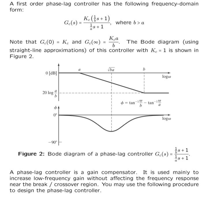
A first order phase-lag controller has the following frequency-domain form: \[ G_{c}(s)=\frac{K_{c}\left(\frac{1}{b} s+1\right)}{\frac{1}{a} s+1} \text {, where } b>a \] Note that \( G_{c}(0)=K_{c} \) and \( G_{c}(\infty)=\frac{K_{c} a}{b} \). The Bode diagram (using straight-line approximations) of this controller with \( K_{c}=1 \) is shown in Figure 2. Figure 2: Bode diagram of a phase-lag controller \( G_{c}(s)=\frac{\frac{1}{b} s+1}{\frac{1}{a} s+1} \). A phase-lag controller is a gain compensator. It is used mainly to increase low-frequency gain without affecting the frequency response near the break / crossover region. You may use the following procedure to design the phase-lag controller. 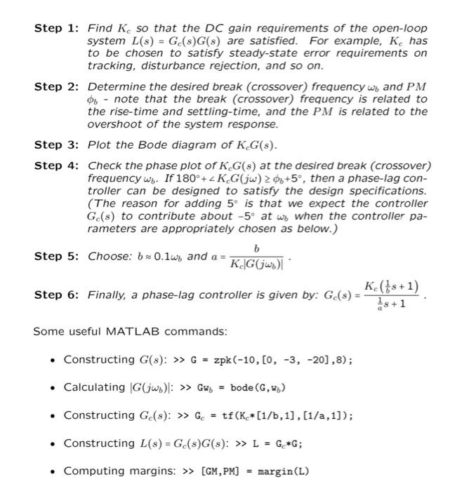Step 1: Find \( K_{c} \) so that the DC gain requirements of the open-loop system \( L(s)=G_{c}(s) G(s) \) are satisfied. For example, \( K_{c} \) has to be chosen to satisfy steady-state error requirements on tracking, disturbance rejection, and so on. Step 2: Determine the desired break (crossover) frequency \( \omega_{b} \) and \( P M \) \( \phi_{b} \) - note that the break (crossover) frequency is related to the rise-time and settling-time, and the \( P M \) is related to the overshoot of the system response. Step 3: Plot the Bode diagram of \( K_{c} G(s) \). Step 4: Check the phase plot of \( K_{c} G(s) \) at the desired break (crossover) frequency \( \omega_{b} \). If \( 180^{\circ}+\angle K_{c} G(j \omega) \geq \phi_{b}+5^{\circ} \), then a phase-lag controller can be designed to satisfy the design specifications. (The reason for adding \( 5^{\circ} \) is that we expect the controller \( G_{c}(s) \) to contribute about \( -5^{\circ} \) at \( \omega_{b} \) when the controller parameters are appropriately chosen as below.) Step 5: Choose: \( b \approx 0.1 \omega_{b} \) and \( a=\frac{b}{K_{c}\left|G\left(j \omega_{b}\right)\right|} \). Step 6: Finally, a phase-lag controller is given by: \( G_{c}(s)=\frac{K_{c}\left(\frac{1}{b} s+1\right)}{\frac{1}{a} s+1} \). Some useful MATLAB commands: - Constructing \( G(s): \gg \mathrm{G}=\mathrm{zpk}(-10,[0,-3,-20], 8) \); - Calculating \( \left|G\left(j \omega_{b}\right)\right|: \gg \mathrm{Gw}_{b}= \) bode \( \left(\mathrm{G}, \mathrm{w}_{b}\right) \) - Constructing \( G_{c}(s): \gg \mathrm{G}_{c}=\operatorname{tf}\left(\mathrm{K}_{c} *[1 / \mathrm{b}, 1],[1 / \mathrm{a}, 1]\right) \); - Constructing \( L(s)=G_{c}(s) G(s): \gg \mathrm{L}=\mathbf{G}_{c} * \mathrm{G} \); - Computing margins: >> [GM,PM] \( =\operatorname{margin}(\mathrm{L}) \) Consider the unity feedback system shown in Figure 1 with: \[ G(s)=\frac{8(s+10)}{s(s+3)(s+20)} \] By following the Algorithm detailed below in the background section, you are required (with the aid of MATLAB) to design a Phase-Lag controller \( G_{C}(s) \) so that the following specifications of the loop transfer function L(s)=Gc(s)G(s)has: A) A phase margin PM \( \geq \mathbf{4 7} \), and a break (crossover) frequency \( \boldsymbol{\omega b}_{\mathbf{b}}=\mathbf{2} . \mathbf{0} \mathrm{rad} / \mathrm{sec} \). B) The steady-state error with respect to a ramp input \( \left(1 / \underline{K}_{v}\right) \) is no greater than \( 0.05 \), where \( \underline{K}_{\text {w }} \) is the velocity error constant. Plot the Bode diagram of the compensated loop transfer function \( G_{c}(s) G(s) \) and validate the frequency domain specification given in part (a). Finally, verify that the step response of the compensated closed-loop system \[ H_{y r}=\frac{G G_{c}}{1+G_{c}} \] will result in a maximum overshoot of no more than \( 20 \% \) and a maximum settling time of 8 seconds.